Understanding Multi-Dimensional Measurement: From Factor Analysis to Cluster Analysis. Multidimensional measurement employs techniques such as factor analysis (FA) to reduce the number of variables to underlying factors (latent constructs) and cluster analysis (CA) to group observations (people/objects) into homogeneous segments.
From Factor Analysis to Cluster Analysis: Understanding Multi-Dimensional Measurement
Introduction: Why Patterns Matter
However limited our knowledge of astronomy, most of us have learned to pick out certain clustering’s of stars from the infinity of those that crowd the northern skies and to name them as the familiar Plough, Orion, and the Great Bear Few of us would identify constellations in the southern hemisphere that are instantly recognizable by those in Australia. Our predilection for reducing the complexity of elements that constitute our lives to a more simple order doesn’t stop at star gazing.
In numerous ways, each and every one of us attempts to discern patterns or shapes in seemingly unconnected events in order to better grasp their significance for us in the conduct of our daily lives. The educational researcher is no exception. As research into a particular aspect of human activity progresses, the variables being explored frequently turn out to be more complex than was first realized. Investigation into the relationship between teaching styles and pupil achievement is a case in point.
Global distinctions between behavior identified as progressive or traditional, informal or formal, are vague and woolly and have led inevitably to research findings that are at worse inconsistent, at best, inconclusive. In reality, epithets such as informal or formal in the context of teaching and learning relate to ‘multi-dimensional concepts’, that is, concepts made up of a number of variables. ‘Multi-dimensional scaling’, on the other hand, is a way of analyzing judgements of similarity between such variables in order that the dimensionality of those judgements can be assessed (Bennett and Bowers, 1977).
As regards research into teaching styles and pupil achievement, it has been suggested that multi-dimensional typologies of teacher behaviour should be developed. Such typologies, it is believed, would enable the researcher to group together similarities in teachers’ judgements about specific aspects of their classroom organization and management, and their ways of motivating, assessing and instructing pupils. Techniques for grouping such judgements are many and various.
What they all have in common is that they are methods for ‘determining the number and nature of the underlying variables among a large number of measures’, a definition which Kerlinger (1970) uses to describe one of the best-known grouping techniques, ‘factor analysis’.
We begin the topic by illustrating a number of methods of grouping or clustering variables ranging from elementary link age analysis which can be undertaken by hand, to factor analysis, which is best left to the computer. We then outline one way of analyzing data cast into multi-dimensional tables. Finally, we append a brief note on a recent, sophisticated technique for exploring multivariate data.
Elementary Linkage Analysis
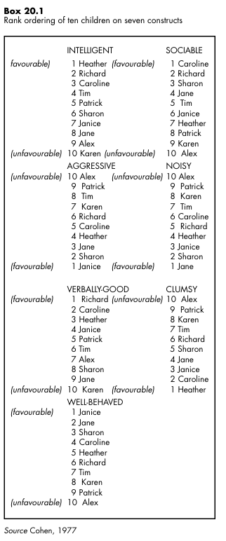
Seven constructs were elicited from an infant school teacher who was invited to discuss the ways in which she saw the children in her class.She identified favorable and unfavorable constructs as follows: ‘intelligent’ (+), ‘sociable’ (+), ‘verbally good’ (+), ‘well-be haved’ (+), ‘aggressive’ (-), ‘noisy’ (-) and ‘clumsy’ (-).
Understanding the Basics
Four boys and six girls were then selected at random from the class register and the teacher was asked to place each child in rank order under each of the seven constructs, using rank position 1 to indicate the child most like the particular construct, and rank position 10, the child least like the particular construct. The teacher’s rank ordering is set out in Picture20.1. Notice that on three constructs, the rankings have been re versed in order to maintain the consistency of favorable 1, unfavorable 10.
Elementary linkage analysis (McQuitty, 1957) is one way of exploring the relationship between the teachers’s personal constructs, that is, of assessing the dimensionality of the judgements that she makes about her pupils. It seeks to identify and define the clustering’s of certain variables within a set of variables. Like factor analysis which we shortly illustrate, elementary linkage analysis searches for interrelated groups of correlation co-efficient.
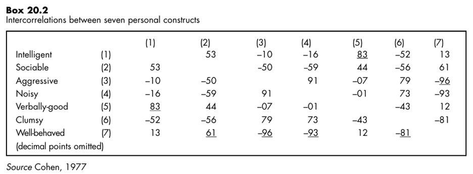
The objective of the search is to identify ‘types’. By type, McQuitty refers to ‘a category of people or other objects (personal constructs in our example) such that the members are internally self-contained in being like one another’. Picture20.2 sets out the intercorrelations between the seven personal construct ratings shown in Picture20.1 (Spearman’s rho is the method of correlation used in this example).
Step-by-Step Process
1 In Picture20.2, underline the strongest that is the highest, correlation co-efficient in each column of the matrix. Ignore negative signs.
2 Identify the highest correlation co-efficient in the entire matrix. The two variables having this correlation constitute the first two of Cluster 1.
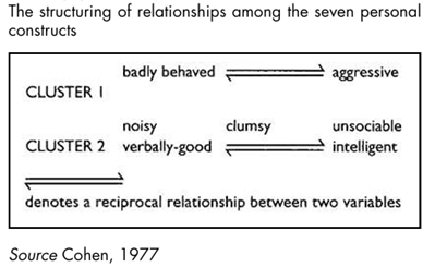
3 Now identify all those variables which are most like the variables in Cluster 1. To do this, read along the rows of the variables which emerged in Step 2, selecting any of the co-efficient which are underlined in the rows. Picture20.3 illustrates diagrammatically the ways in which these new cluster members are related to the original pair which initially constituted Cluster 1. 4 Now identify any variables which are most like the variables elicited in Step 3. Repeat
this procedure until no further variables are identified. 5 Excluding all those variables which belong within Cluster 1, repeat Steps 2 to 4 until all the variables have been accounted for. Cluster analysis: an example1 Elementary linkage analysis is one method of grouping or clustering together correlation co efficient which show similarities among a set of variables.
We now illustrate another method of clustering which was used by Bennett (1976)2 in his study of teaching styles and pupil progress. His starting point was disaffection for global descriptions such as ‘progressive’ and ‘traditional as applied to teaching styles in junior school classrooms.
A more adequate theoretical and experimental conceptualization of the elements constituting teaching styles was attempted through the construction of a questionnaire containing twenty-eight statements illustrating six major areas of teacher classroom behavior: classroom management and control; teacher control and sanctions; curriculum content and planning; instructional strategies; motivational techniques; and assessment procedures.
Bennett constructed a typology of teaching styles from the responses of 468 top-junior school class teachers to the questionnaire. His cluster analysis of their responses involved calculating co-efficient of similarity between subjects across all the variables that constituted the final version of the questionnaire. This technique involves specifying the number of clusters of subjects to which the researcher wishes the data to be reduced.
Examination of the central pro files of all solutions from twenty-two to three clusters, showed that at the twelve-cluster solution level, between-cluster differences were maximized in relation to within-cluster error (see Bennett, 1976). An essential prerequisite to the clustering technique employed in this study was the use of factor analysis to ensure that the variables were relatively independent of one another and that groups of variables were not over weighted in the analysis.
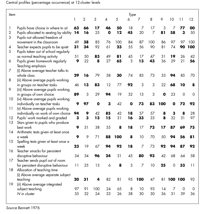
Principal Components analysis followed by varimax rotation reduced the twenty-eight variables in Bennett’s original questionnaire to the nineteen shown in Picture20.4. For purposes of exposition, Bennett ordered the types of teaching style shown in Picture20.4, from the most progressive cluster (Type 1) to the most traditional cluster (Type 12), noting however,
that whilst the extreme types could be described in these terms, the remaining types all contained elements of both progressive and traditional teaching styles. The figures in heavy typeface show percentage response levels that were considered significantly different from the total population distribution.
Cluster Analysis in Teaching Styles Research
1 These teachers favour integration of subject matter, and, unlike most other groups, allow pupils choice of work, whether undertaken individually or in groups. Most allow pupils choice of seating. Less than half curb movement and talk. Assessment in all its forms, tests, grading and homework, appears to be discouraged. Intrinsic motivation is favoured.
2 These teachers also prefer integration of subject matter. Teacher control appears to be low, but less pupil choice of work is offered. However, most allow pupils choice of seating, and only one-third curb movement and talk. Few test or grade work.
3 The main teaching mode of this group is class teaching and group work. Integration of subject matter is preferred, associated with taking pupils out of school. They appear to be strict, most curbing movement and talk, and offenders are smacked. The amount of testing is average, but the amount of grading and homework is below average.
4 These teachers prefer separate subject teaching but a high proportion allow pupil choice both in group and individual work. None seat their pupils by ability. They test and grade more than average.
5 A mixture of separate subject and integrated subject teaching is characteristic of this group. The main teaching mode is pupils working in groups of their own choice on tasks set by the teacher. Teacher talk is lower than average. Control is high with regard to movement but not to talk. Most give tests every week and many give homework regularly. Stars are rarely used, and pupils are taken out of school regularly.
6 These teachers prefer to teach subjects separately with emphasis on groups working on teacher-specified tasks. The amount of individual work is small. These teachers appear to be fairly low on control, and are below average on assessment and the use of extrinsic motivation.
7 This group is separate subject oriented, with a high level of class teaching together with individual work. Teacher control appears to be tight, few allow movement or choice of seating, and offenders are smacked. Assessment, however, is low.
8 This group of teachers has very similar characteristics to those in Type 3, the difference being that these prefer to organize the work on an individual rather than group basis. Freedom of movement is restricted, and most expect pupils to be quiet.
9 These teachers favour separate subject teaching, the predominant teaching mode being individuals working on tasks set by the teacher. Teacher control appears to be high; most curb movement and talk, and seat by ability. Pupil choice is minimal. Regular spelling tests are given, but few mark or grade work or use stars.
10 All these teachers favour separate subject teaching. The teaching mode favoured is teacher talk to whole class, and pupils working in groups determined by the teacher on tasks set by the teacher. Most curb movement and talk, and over two-thirds smack for disruptive behaviour. There is regular testing and most give stars for good work.
11 All members of this group stress separate subject teaching by way of class teaching and individual work. Pupil choice of work is minimal, although most teachers allow choice of seating. Movement and talk are curbed, and offenders smacked.
12 This is an extreme group in a number of respects. None favour an integrated approach. Subjects are taught separately by class teaching and individual work. None allow pupils’ choice of seating and every teacher curbs movement and talk. These teachers are above average on all assessment procedures, and extrinsic motivation predominates.
Bennett’s typology of teacher styles and his analysis of pupil performance based on the typology aroused considerable debate. Readers may care to follow up critical comments on the cluster analysis procedures we have outlined here.3 It is important to note, perhaps, how times have changed since this study was undertaken— many of the practices that Bennett describes would be considered illegal today!
Bennett’s Groundbreaking Study
Factor analysis, we said earlier, is a way of determining the nature of underlying patterns among a large number of variables. It is particularly appropriate in research where investigators aim to impose an ‘orderly simplification’ (Child, 1970) upon a number of interrelated measures. We illustrate the use of factor analysis in a study of occupational stress among teachers (McCormick and Solman, 1992).
The 12 Teaching Style Types
Despite a decade or so of sustained research, the concept of occupational stress still causes difficulties for researchers intent upon obtaining objective measures in such fields as the physiological and the behavioral, because of the wide range of individual differences. Moreover, subjective measures such as self-reports, by their very nature, raise questions about the external validation of respondents’ revelations.
This latter difficulty notwithstanding, McCormick and Solman (1992) chose the methodology of self-report as the way into the problem, dichotomizing it into first, the teacher’s view of self, and second, the external world as it is seen to impinge upon the occupation of teaching. Stress, according to the researchers, is considered as ‘an unpleasant and unwelcome emotion’ whose negative effect for many is ‘associated with illness of varying degree’ (McCormick and Solman, 1992). They began their study on the basis of the following premises:
1 Occupational stress is an undesirable and negative response to occupational experiences.
2 To be responsible for one’s own occupational stress can indicate a personal failing.
Drawing on attribution theory, McCormick and Solman consider that the idea of blame is a key element in a framework for the exploration of occupational stress. The notion of blame for occupational stress, they assert, fits in well with tenets of attribution theory, particularly in terms of attribution of responsibility having a self-serving bias.
Taken in concert with organizational facets of schools, the researchers hypothesized that teachers would ‘externalize responsibility for their stress increasingly to increasingly distant and identifiable domains’ (McCormick and Solman, 1992). Their selection of dependent and independent variables in the research followed directly from this major hypothesis. McCormick and Solman developed a questionnaire instrument that included thirty-two items to do with occupational satisfaction.
These were scored on a continuum ranging from ‘strongly disagree’ to ‘strongly agree’. Thirty eight further items had to do with possible sources of occupational stress. Here, respondents rated the intensity of the stress they experienced when exposed to each source. Stress items were judged on a scale ranging from ‘no stress’ to ‘extreme stress’. In yet another section of the questionnaire, respondents rated how responsible they felt certain nominated persons or institutions were for the occupational stress that they, the respondents, experienced.
These entities included self, pupils, superiors, the Department of Education, the Government and society itself. Finally, the teacher-participants were asked to complete a fourteen-item Locus of Control scale, giving a measure of internality/externality. ‘Internals’ are people who see outcomes as a function of what they themselves do; ‘externals’ see outcomes as a result of forces beyond their control.
The items included in this lengthy questionnaire arose partly from statements about teacher stress used in earlier investigations, but mainly as a result of hunches about blame for occupational stress that the researchers derived from attribution theory. As Child (1970) observes: In most instances, the factor analysis is preceded by a hunch as to the factors that might emerge. In fact, it would be difficult to conceive of a manageable analysis which started in an empty-headed fashion…
Even the ‘let’s see what happens’ approach is pretty sure to have a hunch at the back of it somewhere. It is this testing and the generation of hypotheses which forms the principal concern of most factor analysts. (Child, 1970).
The 90-plus-item inventory was completed by 387 teachers. Separate correlation matrices com posed of the inter-correlations of the 32 items on the satisfaction scale, the 8 items in the persons/institutions responsibility measure and the 38 items on the stress scale were factor analysed. The technical details of factor analysis are beyond the scope of this and previous topics . Briefly, however, the procedures followed by McCormick and Solman involved a method called Principal Components, by means of which factors or groupings are extracted.
These are rotated to produce a more meaningful interpretation of the under lying structure than that provided by the Principal Components method. (Readable accounts of factor analysis may be found in Kerlinger (1970) and Child (1970).) In the factor analysis of the eight-item responsibility for stress measure, the researchers identified three factors. Picture20.5 shows those three factors with what are called their ‘factor loadings’. These are like correlation co-efficients, ranging from -1.0 to +1.0 and are interpreted similarly. That is to say they indicate the correlation between the person/institution responsibility items shown in Picture20.5, and the factors.
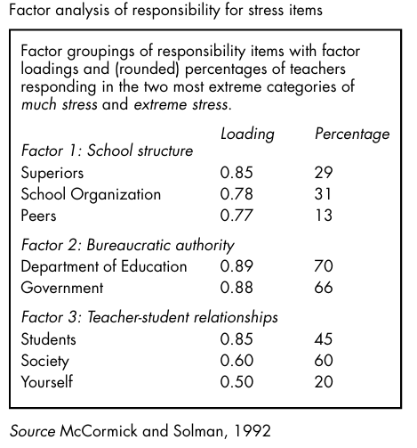
Looking at Factor 1, ‘School structure’, for ex ample, it can be seen that in the three items loading there are, in descending order of weight, superiors (0.85), school organization (0.78) and peers (0.77). ‘School structure’ as a factor, the authors suggest, is easily identified and readily explained.
But what of Factor 3, ‘Teacher—student relationships’, which includes the variables students, society and yourself? McCormick and Solman (1992) proffer the following tentative interpretation: An explanation for the inclusion of the variable ‘yourself’ in this factor is not readily at hand. Clearly, the difference between the variable ‘yourself and the ‘students’ and ‘society’ variables is that only 20% of these teachers rated themselves as very or extremely responsible for their own stress, compared to 45% and 60% respectively for the latter two.
Possibly the degree of responsibility which teachers attribute to themselves for their occupational stress is associated with their perceptions of their part in controlling student behaviour. This would seem a reasonable explanation, but requiring further investigation. (McCormick and Solman, 1992) Picture20.6 shows the factors derived from the analysis of the thirty-eight occupational stress items. Five factors were extracted. They were named: ‘Student domain’, ‘External (to school) domain’, ‘Time demands’, ‘School domain’ and ‘Personal domain’.
Whilst a detailed discussion of the factors and their loadings is inappropriate here, we draw readers’ attention to one or two interesting findings. Notice, for example, how the second factor, ‘External (to school) domain’, is consistent with the factoring of the responsibility for stress items reported in Picture20.5.
That is to say, the variables to do with the Government and the Department of Education have loaded on the same factor. The researchers venture this further elaboration of the point: when a teacher attributes occupational stress to the Department of Education, it is not as a member of the Department of Education, although such, in fact is the case.
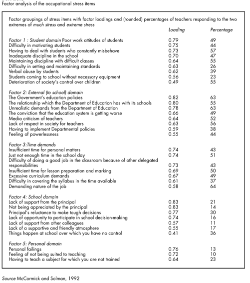
In this context, the Department of Education is outside ‘the system to which the teacher belongs’, namely the school. A similar argument can be posed for the nebulous concept of Society. The Government is clearly a discrete political structure. (McCormick and Solman, 1992) ‘School domain’, Factor 4 in Picture20.6, consists of items concerned with support from the school principal and colleagues as well as the general nurturing atmosphere of the school.
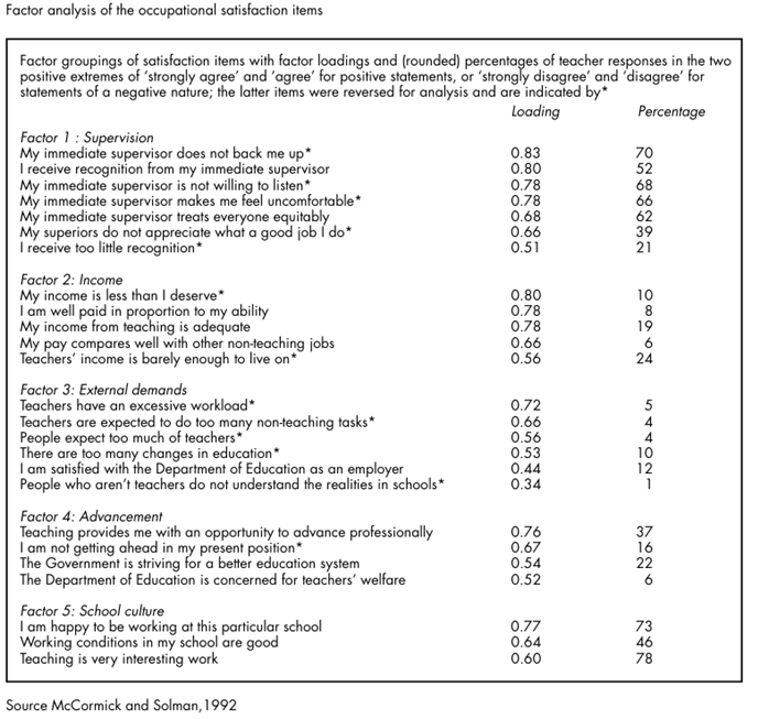
Of particular interest here is that teachers report relatively low levels of stress for these items. Picture20.7 reports the factor analysis of the thirty-two items to do with occupational satisfaction. Five factors were extracted and named as ‘Supervision’, ‘Income’, ‘External demands’, ‘Advancement’ and ‘School culture’. Again, space precludes a full outline of the results set out in Picture20.7.
Notice, however, an apparent anomaly in the first factor, ‘Supervision’. Responses to items to do with teachers’ supervisors and recognition seem to indicate that in general, teachers are satisfied with their supervisors, but feel that they receive too little recognition. Picture20.7 shows that 21 per cent of teacher-respondents agree or strongly agree that they receive too little recognition, yet 52 per cent agree or strongly agree that they do receive recognition from their immediate supervisors.
McCormick and Solman offer the following explanation: The difference can be explained, in the first instance, by the degree or amount of recognition given. That is, immediate supervisors give recognition, but not enough. Another interpretation is that superiors other than the immediate supervisor do not give sufficient recognition for their work. (McCormick and Solman, 1992) Here is a clear case for some form of respondent validation.
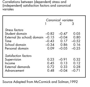
Having identified the underlying structures of occupational stress and occupational satisfaction, the researchers then went on to explore the relationships between stress and satisfaction by using a technique called ‘canonical correlation analysis’. The technical details of this procedure are beyond the scope of this and previous topics. Interested readers are referred to Levine, who suggests that ‘the most acceptable approach to interpretation of canonical variates is the examination of the correlations of the original variables with the canonical variate’ (Levine, 1984).
This is the procedure adopted by McCormick and Solman. From Picture20.8 we see that factors having high correlations with Canonical Variate 1 are Stress: Student domain (-0.82) and Satisfaction: External demands (0.72). The researchers offer the following interpretation of this finding: [This] indicates that teachers perceive that ‘non teachers’ or outsiders expect too much of them (External demands) and that stress results from poor student attitudes and behaviour (Student domain).
One interpretation might be that for these teachers, high levels of stress attributable to the Student domain are associated with low levels of satisfaction in the context of demands from outside the school, and vice versa. It may well be that, for some teachers, high demand in one of these is perceived as affecting their capacity to cope or deal with the demands of the other.
Certainly, the teacher who is experiencing the urgency of a struggle with student behaviour in the classroom, is unlikely to think of the requirements of persons and agencies outside the school as important. (McCormick and Solman, 1992) The outcomes of their factor analyses frequently puzzle researchers. Take, for example, one of the loadings on the third canonical variate. There, we see that the stress factor ‘Time demands’ correlates negatively (-0.52).
One might have supposed, the authors say, that stress attributable to the external domain would have correlated with the variate in the same direction. But this is not so. It correlates positively at 0.80. One possible explanation, they suggest, is that an increase in stress experienced because of time demands coincides with a lowering of stress attributable to the external domain, as time is expended in meeting demands from the external domain. The researchers concede, however, that this explanation would need close examination before it could be accepted.

Critical Considerations
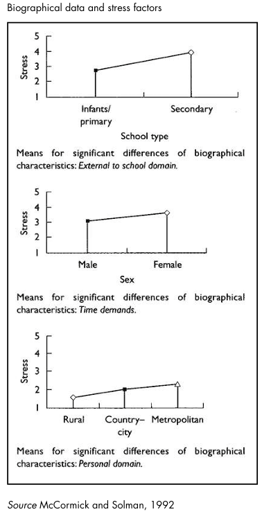
McCormick and Solman’s questionnaire also elicited biographical data from the teacher-respondents in respect of sex, number of years teaching, type and location of school and position held in school. By rescoring the stress items on a scale ranging from ‘No stress’ (1) to ‘Extreme stress’ (5) and using the means of the factor scores, the researchers were able to explore associations between the degree of perceived occupational stress and the biographical data supplied by participants. Space precludes a full account of McCormick and Solman’s findings. We illustrate two or three significant results in Picture20.9.
In the School domain more stress was reported by secondary school teachers than by their colleagues teaching younger pupils, not really a very surprising result, the researchers observe, given that infant/primary schools are generally much smaller than their secondary counterparts and that teachers are more likely to be part of a smaller, supportive group. In the domain of Time demands, females experienced more stress than males, a finding consistent with that of other research.
In the Personal domain, a significant difference was found in respect of the school’s location, the level of occupational stress increasing from the rural setting, through the country/city to the metropolitan area. To conclude, factor analysis techniques are ideally suited to studies such as that of McCormick and Solman in which lengthy questionnaire-type data are elicited from a large number of participants and where researchers are concerned to explore underlying structures and relationships between dependent and independent variables. Inevitably, such tentative explorations raise as many questions as they answer.
Factor Analysis: Exploring Teacher Stress
The use of factor analysis and linkage analysis in studies of children’s judgements of educational situations is illustrated in the work of Magnusson (1971) and Ekehammar and Magnusson (1973). In the latter study, pupils were required to rate descriptions of various educational episodes on a scale of perceived similarity ranging from ‘0=not at all similar’ to ‘4=identical’. Twenty different situations were presented, two at a time, in the same randomized order for all subjects. For example, ‘listening to a lecture but do not understand a thing’ would be judged against ‘sitting at home writing an essay’.
Product moment correlation co-efficients between pairs of similarity matrices calculated for all subjects varied between 0.57 and 0.79, with a median value of 0.71. No individual matrix deviated markedly from any of the others. A factor analysis of the total correlation matrix showed that the descriptions of situations had very clear structures for the children involved. Moreover, judgements of perceived similarity between situations had a considerable degree of consistency over time. Ekehammar and Magnusson (1973) compared their dimensional analysis with a categorical approach to the data using elementary linkage (McQuitty, 1957).
They reported that this latter approach gave a result which was entirely in agreement with the result of the dimensional analysis. Five categories of situations were obtained with the same situations distributed in categories in the same way as they were distributed in factors in the dimensional analysis.
What is Factor Analysis?
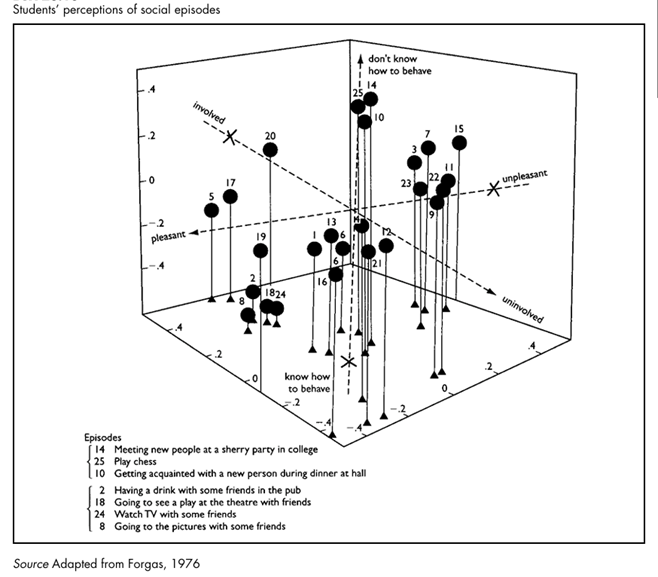
Forgas (1976) studied housewives’ and students’ perceptions of typical social episodes in their lives, the episodes having been elicited from the respective groups by means of a diary technique. Subjects were required to supply two adjectives to describe each of the social episodes they had recorded as having occurred during the previous twenty-four hours. From a pool of some 146 adjectives thus generated, ten (together with their antonyms) were selected on the basis of their salience, their diversity of usage and their independence of one another. Two more scales from speculative taxonomies were added to give twelve uni-dimensional scales purporting to de scribe the underlying episode structures.
These scales were used in the second part of the study to rate twenty-five social episodes in each group, the episodes being chosen as follows. An ‘index of relatedness’ was computed on the basis of the number of times a pair of episodes was placed in the same category by respective house-wife and student judges. Data were aggregated over the total number of subjects in each of the two groups. The twenty-five ‘top’ social episodes in each group were retained.
Forgas’s analysis is based upon the ratings of twenty-six housewives and twenty-five students of their respective twenty-five episodes on each of the twelve uni dimensional scales. Picture20.10 shows a three dimensional configuration of twenty-five social episodes rated by the student group on three of the scales. For illustrative purposes some of the social episodes numbered in Picture20.10 are identified by specific content.
In another study, Forgas examined the social environment of a university department consist ing of tutors, students and secretarial staff, all of whom had interacted both inside and outside the department for at least six months prior to the research and thought of themselves as an intensive and cohesive social unit. Forgas’s interest was in the relationship between two aspects of the social environment of the department—the perceived structure of the group and the perceptions that were held of specific social episodes.
Participants were required to rate the similarity between each possible pairing of group members on a scale ranging from ‘1= extremely similar’ to ‘9=extremely dissimilar’. An individual differences multi-dimensional scaling procedure (INDSCAL) produced an optimal three dimensional configuration of group structure accounting for 68 per cent of the variance, group members being differentiated along the dimensions of sociability, creativity and competence.
A semi-structured procedure requiring participants to list typical and characteristic inter action situations were used to identify a number of social episodes. These in turn were validated by participant observation of the ongoing activities of the department.
The most commonly occurring social episodes (those mentioned by nine or more members) served as the stimuli in the second stage of the study. Bi-polar scales similar to those reported by Forgas (1976) and elicited in like manner were used to obtain group members’ judgements of social episodes. An interesting finding reported by Forgas was that formal status differences exercised no significant effect upon the perception of the group by its members, the absence of differences being attributed to the strength of the department’s cohesiveness and intimacy.
In Forgas’s analysis of the group’s perceptions of social episodes, the INDSCAL scaling procedure produced an optimal four-dimensional solution accounting for 62 per cent of the variance, group members perceiving social episodes in terms of anxiety, involvement, evaluation and social-emotional versus task orientation.
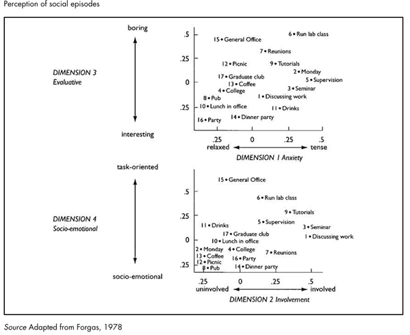
Picture20.11 illustrates how an average group member would see the characteristics of various social episodes in terms of the dimensions by which the group commonly judged them. Finally we outline a classificatory system that has been developed to process materials elicited in a rather structured form of account gathering.
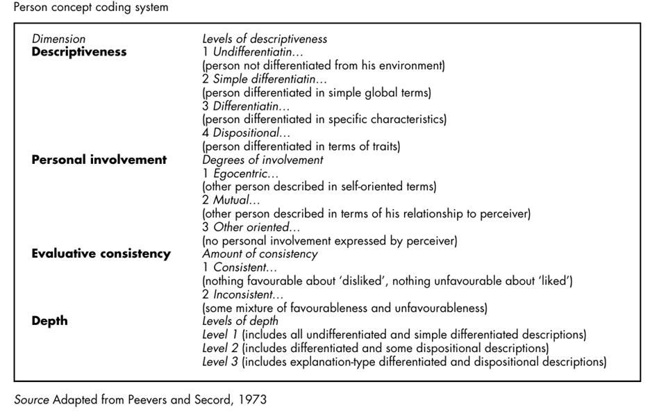
Peevers and Secord’s study of developmental changes in children’s use of descriptive concepts of persons, illustrates the application of quantitative techniques to the analysis of one form of account. In individual interviews, children of varying ages were asked to describe three friends and one person whom they disliked, all four people being of the same sex as the interviewee. Interviews were tape-recorded and transcribed.
A person-concept coding system was developed, the categories of which are illustrated in Picture20.12. Each person description was divided into items, each item consisting of one discrete piece of information. Each item was then coded on each of four major dimensions. Detailed coding procedures are set out in Peevers and Secord (1973).
Tests of inter judge agreement on descriptive ness, personal involvement and evaluative consistency in which two judges worked independently on the interview transcripts of twenty-one boys and girls aged between five and sixteen years resulted in interjudge agreement on those three dimensions of 87 per cent, 79 per cent and 97 per cent respectively. Peevers and Secord also obtained evidence of the degree to which the participants themselves were consistent from one session to another in their use of concepts to describe other people.
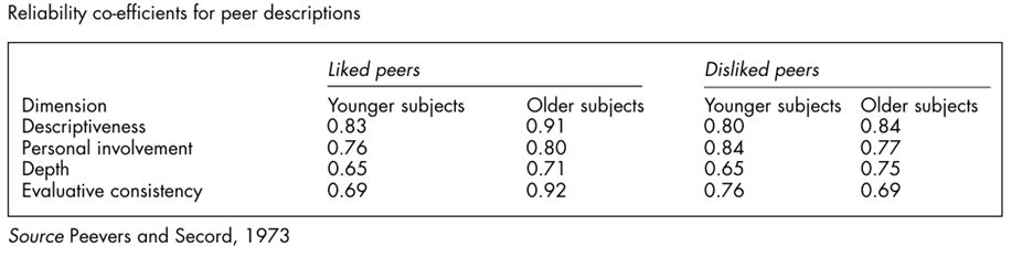
Children were reinter viewed between one week and one month after the first session on the pre text of problems with the original recordings. Indices of test-retest reliability were computed for each of the major coding dimensions. Separate correlation co-efficients (eta) were obtained for younger and older children in respect of their descriptive concepts of liked and disliked peers.
Reliability co-efficients are as set out in Picture20.13. Secord and Peevers (1974) conclude that their approach offers the possibility of an exciting line of inquiry into the depth of insight that individuals have into the personalities of their acquaintances. Their ‘free commentary’ method is a modification of the more structured interview, requiring the interviewer to probe for explanations of why a person behaves the way he or she does or why a person is the kind of person he or she is.
Peevers and Secord found that older children in their sample readily volunteered this sort of information. Harré (1977b) observes that this approach could also be ex tended to elicit commentary upon children’s friends and enemies and the ritual actions associated with the creation and maintenance of these categories.
Working with Multi-Dimensional Tables
A frequently used statistic for a 2×2 contingency table is the chi-square ( ) statistic. The chisquare statistic measures the difference between a statistically generated expected and an actual result to see if there is a significant difference between them, i.e. to see if the frequencies observed are significant; it is a measure of ‘good ness of fit’ between an expected and an actual result or set of results. The expected result is based on a statistical process discussed below.
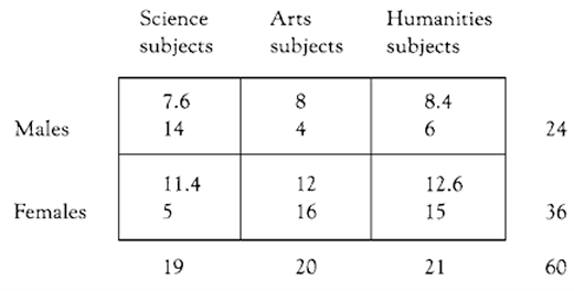
The chi-square statistic addresses the notion of statistical significance, itself based on notions of probability. For a chi-square statistic data are set into a contingency table, an example of which can be seen below, a 2×3 contingency table, i.e. two horizontal rows and three columns (contingency tables may contain more than this number of variables). The example in this figure presents data concerning sixty students’ entry into science, arts and humanities, in a college, and whether the students were male or female (Morrison, 1993:132–4).
The lower of the two figures in each cell is the number of actual students who have opted for the particular subjects (sciences, arts, humanities). The upper of the two figures in each cell is what might be expected purely by chance to be the number of students opting for each of the particular subjects. The figure is arrived at by statistical computation, hence the decimal fractions for the figures. What is of interest to the researcher is whether the actual distribution of subject choice by males and females differs significantly from that which could occur by chance variation in the population of college entrants.
The researcher begins with the hypothesis that there is no significant difference between the actual results noted and what might be expected to occur by chance in the wider population (the null hypothesis). When the chi-square statistic is calculated, if the observed, actual distribution differs from that which might be expected to occur by chance alone, then the researcher has to deter mine whether that difference is statistically significant, i.e. to reject the null hypothesis.
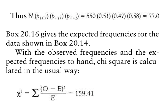
Our example using sixty students, using a chisquare formula (available in most books on statistics) yields a final chi-square figure of 14.64; this is the figure computed from the sample of 60 college entrants. The researcher then refers to tables of the distribution of chi-square (given in most books on social science statistics) and looks up the figure to see if it indicates a statistically significant difference from that occurring by chance. Part of the chi-square distribution table is shown here:
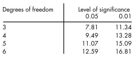
The researcher will see that the ‘degrees of freedom’ (a mathematical construct that is related to the number of restrictions that have been placed on the data) have to be identified. In many cases, to establish the degrees of freedom, one simply takes 1 away from the total number of rows of the contingency table and 1 away from the total number of columns and adds them; in this case it is (2–1)+(3–1)=3 degrees of freedom. Degrees of freedom are discussed later in this topic. (Other formulae for ascertaining degrees of freedom hold that the number is the total number of cells minus one—this is the method set out later in this chapter.)
In our example above, the researcher looks along the table from the entry for the three degrees of freedom and notes that the figure calculated—of 14.64—is statistically significant at the 0.01 level, i.e. is higher than the required 11.34, indicating that the results obtained—the distributions of the actual data—could not have occurred simply by chance. The null hypothesis is rejected at the 0.01 level of significance.
Interpreting the specific figures of the contingency table in educational rather than statistical terms, noting:
(a) the low incidence of females in the science subjects and the high incidence of females in the arts and humanities subjects
(b) the high incidence of males in the science subjects and low incidence of males in the arts and humanities, the researcher would say that this distribution is significant—suggesting, perhaps, that the college needs to consider action possibly to encourage females into science subjects and males into arts and humanities.
There are numerous statistical packages available for computer use that will process the calculations for most researchers; they will simply need to enter the raw data and the computer will process the data and indicate the level of statistical significance of the distributions. A much-used package is the Statistical Package for Social Sciences (SPSS) which will process these data using the CROSSTABS command sequence.
The chi-square test requires at least 80 per cent of the cells of a contingency table to contain at least five cases if confidence is to be placed in the results. This means that it may not be feasible to calculate the chi-square statistic if only a small sample is being used. Hence the re searcher would tend to use this statistic for larger-scale survey data. Other approaches could be used if the problem of low cell frequencies obtains (Cohen and Holliday, 1996).
Methods of analyzing data cast into 2×2 contingency tables by means of the chi square test are generally well covered in research methods books. Increasingly, however, educational data are classified in multiple rather than two-dimensional formats. Everitt (1977) provides a useful account of methods for analyzing multi-dimensional tables and has shown, incidentally, the erroneous conclusions that can result from the practice of analyzing multi-dimensional data by summing over variables to reduce them to two-dimensional formats.
In this section we too illustrate the misleading conclusions that can arise when the researcher employs bivariate rather than multivariate analysis. The outline that follows draws closely on an exposition by Whiteley (1983).
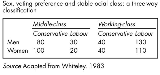
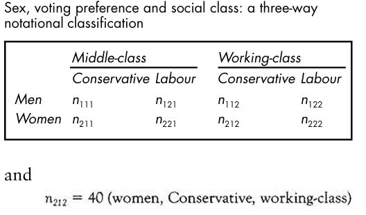
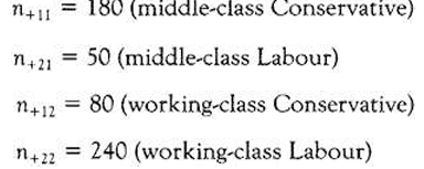
Multi-dimensional data: some words on notation The hypothetical data in Picture20.14 refer to a survey of voting behaviour in a sample of men and women in Britain: the row variable (sex) is represented by i; the column variable (voting preference) is rep resented by j; the layer variable (social class) is represented by k. The number in any one cell in Picture20.14 can be represented by the symbol nijk that is to say, the score in row category i column category j, and layer category k, where:
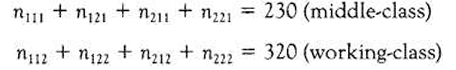
It follows therefore that the numbers in Picture20.14 can also be represented as in Picture20.15. Thus,
Three types of marginal can be obtained from Picture20.15 by:
- Summing over two variables to give the marginal totals for the third.
Thus: n++k =summing over sex and voting preference to give social class, for example:
n+j+ =summing over sex and social class to give voting preference
ni++ =summing over voting preference and social class to give sex.
- Summing over one variable to give the marginal totals for the second and third variables. Thus:
- Summing over all three variables to give the grand total. Thus:
![]()
Using the chi square test in a three way classification table
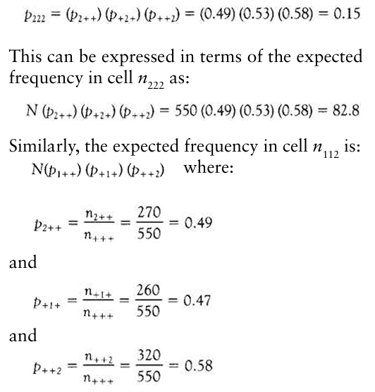
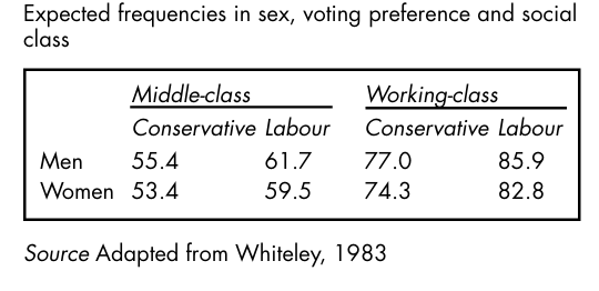
Whiteley (1983) shows how easy it is to extend the 2×2 chi square test to the three-way case. The probability that an individual taken from the sample at random in Picture20.10 will be a woman is:
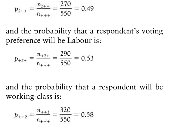
To determine the expected probability of an individual being a woman, Labour supporter and working-class we assume that these variables are statistically independent (that is to say, there is no relationship between them) and simply apply the multiplication rule of probability theory:
![]()
Degrees of freedom
As Whiteley observes, degrees of freedom in a three-way contingency table are more complex than in a 2×2 classification. Essentially, however, degrees of freedom refer to the freedom with which the researcher is able to assign values to the cells, given fixed marginal totals. This can be computed by first determining the degrees of freedom for the marginal. Each of the variables in our example (sex, voting preference, and social class) contains two categories.
It follows therefore that we have (2 1) degrees of freedom for each of them, given that the marginal for each variable is fixed. Since the grand total of all the marginal (i.e. the sample size) is also fixed, it follows that one more degree of freedom is also lost. We subtract these fixed numbers from the total number of cells in our contingency table. In general therefore: degrees of freedom (df)=the number of cells in the table-1 (for N)-the number of cells fixed by the hypothesis being tested.
Thus; where r=rows, c=columns and l=layers:
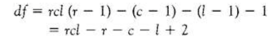
that is to say when we are testing the hypothesis of the mutual independence of the three variables. In our example:
![]()
From chi square tables we see that the critical value of with four degrees of freedom is 9.49 at p=0.05. Our obtained value greatly exceeds that number. We reject the null hypothesis and conclude that sex, voting preference, and social class are significantly interrelated. Having rejected the null hypothesis with respect to the mutual independence of the three variables, the researcher’s task now is to identify which variables cause the null hypothesis to be rejected.
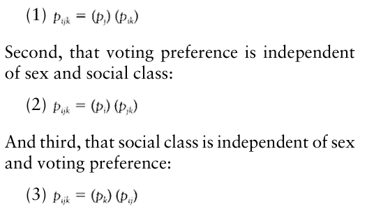
We cannot simply assume that because our chi-square test has given a significant result, it therefore follows that there are significant associations between all three variables. It may be the case, for example, that an association exists between two of the variables whilst the third is completely independent. What we need now is a test of ‘partial independence’.Whiteley shows the following three such possible tests in respect of the data in Picture20.10. First, that sex is independent of social class and voting preference:
The following example shows how to construct the expected frequencies for the first hypothesis.
We can determine the probability of an individual being, say, woman, Labour, and working-class, assuming hypothesis (1), as follows:
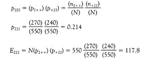
That is to say, assuming that sex is independent of social class and voting preference, the expected number of female, working class Labour supporters is 117.8. When we calculate the expected frequencies for each of the cells in our contingency table in respect of our first hypothesis , we obtain the results shown in Picture20.17.
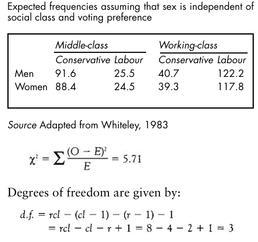
Whiteley observes: Note that we are assuming c and l are interrelated so that once, say, p+11 is calculated, then p+12 , p+21 and p+22 are determined, so we have only 1 degree of freedom; that is to say, we lose (cl-1) degrees of freedom in calculating that relationship. (Whiteley, 1983)
From chi square tables we see that the critical value of with three degrees of freedom is 7.81 at . Our obtained value is less than this. We therefore accept the null hypothesis and conclude that there is no relationship between sex on the one hand and voting preference and social class on the other. Suppose now that instead of casting our data into a three-way classification as shown in Picture20.14, we had simply used a 2×2 contingency table and that we had sought to test the null hypothesis that there is no relationship between sex and voting preference. The data are shown in Picture20.18.
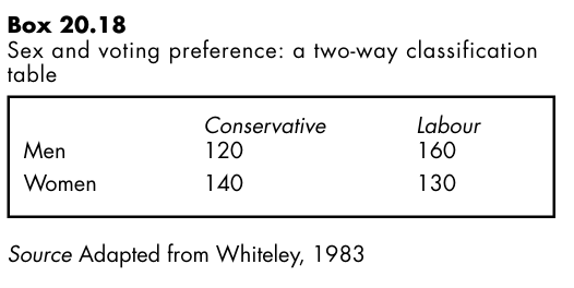
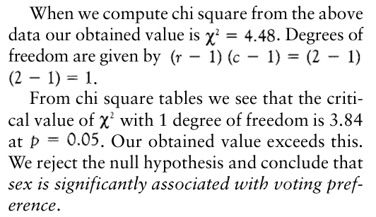
But how can we explain the differing conclusions that we have arrived at in respect of the data in Boxes 20.14 and 20.18? These examples illustrate an important and general point, Whiteley observes. In the bivariate analysis (Picture20.18) we concluded that there was a significant relationship between sex and voting preference. In the multivariate analysis (Picture20.14) that relationship was found to be non-significant when we controlled for social class. The lesson is plain: use a multivariate approach to the analysis of contingency tables wherever the data allow.
Advanced Techniques: Multilevel Modeling
Multilevel modeling (also known as multilevel regression) is a statistical method that recognizes that it is uncommon to be able to assign students in schools randomly to control and ex perimental groups, or indeed to conduct an experiment that requires an intervention with one group whilst maintaining a control group (Keeves and Sellin, 1997:394). Typically in most schools, students are brought together in particular groupings for specified purposes and each group of students has its own different characteristics which render it different from other groups.
Multilevel modelling addresses the fact that, unless it can be shown that different groups of students are, in fact, alike, it is generally inappropriate to aggregate groups of students or data for the purposes of analysis. Indeed multilevel modelling provides a striking critique of Bennett’s (1976) research on teaching styles that we report earlier in this topic (Aitken, Anderson and Hinde, 1981). Multilevel models avoid the pitfalls of aggregation and the ecological fallacy (Plewis, 1997:35), i.e. making inferences about individual students and behaviour from aggregated data.
Data and variables exist at individual and group levels, indeed Keeves and Sellin (1997) break down analysis further into three main levels:
(a) between students over all groups
(b) between groups
(c) between students within groups.
One could extend the notion of levels, of course, to include individual, group, class, school, local, regional, national and international levels (Paterson and Goldstein, 1991). This has been done using multilevel regression and hierarchical linear modelling. Multilevel models en able researchers to ask questions hitherto unanswered, e.g. about variability between and within schools, teachers and curricula (Plewis, 1997:34 5), in short about the processes of teaching and learning.6 Useful overviews of multilevel model ling can be found in Goldstein (1987), Fitz-Gib bon (1997) and Keeves and Sellin (1997).
Multilevel analysis avoids statistical treatments associated with experimental methods (e.g. analysis of variance and covariance); rather, it uses re gression analysis and, in particular, multilevel regression. Regression analysis, argues Plewis (1997:28), assumes homoscedasticity (where the residuals demonstrate equal scatter), that the residuals are independent of each other, and finally, that the residuals are normally distributed.
The whole field of multilevel modelling has proliferated rapidly in the 1990s, and is the basis of much research that is being undertaken on the ‘value added’ component of education and the comparison of schools in public ‘league tables’ of results (Fitz-Gibbon, 1991, 1997). However Fitz Gibbon (1997:42–4) provides important evidence to question the value of some forms of multilevel modelling.
She demonstrates that residual gain analysis provides answers to questions about the value-added dimension of education which differ insubstantially from those answers that are given by multilevel modelling (the lowest correlation co efficient being 0.93 and 71.4 per cent of the correlations computed correlating between 0.98 and 1). The important point here is that residual gain analysis is a much more straightforward technique than multilevel modelling. Her work strikes at the heart of the need to use complex multilevel modelling to assess the ‘value-added’ component of education.
In her work (Fitz-Gibbon, 1997:5) the value-added score—the difference between a statistically predicted performance and the actual performance—can be computed using residual gain analysis rather than multilevel modelling. None the less, multilevel modelling now attracts worldwide interest.
Whereas ordinary regression models do not make allowances, for example, for different schools (Paterson and Goldstein, 1991), multilevel regression can include school differences, and, indeed other variables, for example: socio economic status (Willms, 1992), single and co-educational schools (Daly, 1996; Daly and Shuttleworth, 1997), location (Garner and Raudenbush, 1991), size of school (Paterson, 1991) and teaching styles (Zuzovsky and Aitken, 1991). Indeed Plewis (1991a) indicates how multilevel modelling can be used in longitudinal studies, linking educational progress with curriculum coverage.
Read More:
https://nurseseducator.com/didactic-and-dialectic-teaching-rationale-for-team-based-learning/
https://nurseseducator.com/high-fidelity-simulation-use-in-nursing-education/
First NCLEX Exam Center In Pakistan From Lahore (Mall of Lahore) to the Global Nursing
Categories of Journals: W, X, Y and Z Category Journal In Nursing Education
AI in Healthcare Content Creation: A Double-Edged Sword and Scary
Social Links:
https://www.facebook.com/nurseseducator/
https://www.instagram.com/nurseseducator/
https://www.pinterest.com/NursesEducator/
https://www.linkedin.com/company/nurseseducator/
https://www.linkedin.com/in/nurseseducator/
https://x.com/nurseseducator?t=-CkOdqgd2Ub_VO0JSGJ31Q&s=08
https://www.researchgate.net/profile/Afza-Lal-Din
https://scholar.google.com/citations?hl=en&user=F0XY9vQAAAAJ