Correlational Research Methods: How to Measure and Interpret Variable Relationships

The Correlational Research Methods: How to Measure and Interpret Variable Relationships. Correlational research measures the relationship between two or more variables using methods such as surveys or naturalistic observation, and this relationship is interpreted using a correlation coefficient (r).

What is Correlational Research Methods: How to Measure and Interpret Variable Relationships

A correlation coefficient is a number between -1 and +1, where the sign indicates the direction (positive or negative) and the value indicates the strength of the relationship, but it does not imply causality.

What is Correlational Research?

Human behavior at both the individual and social level is characterized by great complexity, a complexity about which we understand comparatively little, given the present state of social research. One approach to a fuller understanding of human behavior is to begin by teasing out simple relationships between those factors and elements deemed to have some bearing on the phenomena in question. The value of correlational research is that it is able to achieve this end.

Much of social research in general, and educational research more particularly, is concerned at our present stage of development with the first step in this sequence—establishing interrelationships among variables. We may wish to know, for example, how delinquency is related to social class background; or whether an association exists between the number of years spent in full-time education and subsequent annual income; or whether there is a link between personality and achievement.

Numerous techniques have been devised to provide us with numerical representations of such relationships and they are known as ‘measures of association’. We list the principal ones in Box . The interested reader is referred to Cohen and Holliday (1982, 1996), texts containing worked examples of the appropriate use (and limitations) of the correlational techniques outlined in Box , together with other measures of association such as Kruskal’s gamma, Somer’s d, and Guttman’s lambda.

Understanding Variables and Scales of Measurement

Look at the words used at the top of the Box to explain the nature of variables in connection with the measure called the Pearson product roment, r. The variables, we learn, are ‘continuous’ and at the ‘interval’ or the ‘ratio’ scale of measurement.

Continuous Variables and Ratio Scales

A continuous variable is one that, theoretically at least, can take any value between two points on a scale. Weight, for ex ample, is a continuous variable; so too is time, so also is height. Weight, time and height can take on any number of possible values between bought and infinity, the feasibility of measuring them across such a range being limited only by the variability of suitable measuring instruments. A ratio scale includes an absolute zero and pro vides equal intervals.

Using weight as our example, we can say that no mass at all is a zero measure and that 1,000 grams is 400 grams heavier than 600 grams and twice as heavy as 500. In our discussion of correlational research that follows, we refer to a relationship as a ‘correlation’ rather than an ‘association’ whenever that relationship can be further specified in terms of an increase or a decrease of a certain number of units in the one variable (IQ for example) producing an increase or a decrease of a related number of units of the other (e.g. mathematical ability).

Ordinal Scales and Rank Order

Turning again to Box , we read in connection with the second measure shown there (Rank order or Kendall’s tau) that the two continuous variables are at the ‘ordinal’ scale of measurement. An ordinal scale is used to indicate rank order; that is to say, it arranges individuals or objects in a series ranging from the highest to the lowest according to the particular characteristic being measured. In contrast to the interval scale discussed earlier, ordinal numbers assigned to such a series do not indicate absolute quantities nor can one assume that the intervals between the numbers are equal.

For example, in a class of children rated by a teacher on the degree of their co-cooperativeness and ranged from highest to lowest according to that attribute, it cannot be assumed that the difference in the degree of co-cooperativeness between subjects ranked 1 and 2 is the same as that obtaining between subjects 9 and 10; nor can it be taken that subject 1 possesses 10 times the quantity of co-cooperativeness’ of subject 10.

Nominal Scales and Dichotomous Variables

The variables involved in connection with the phi co-efficient measure of association (halfway down Box ) are described as ‘true dichotomies’ and at the ‘nominal’ scale of measurement. Truly dichotomous variables (such as sex or driving test result) can take only two values (male or female; pass or fail). The nominal scale is the most elementary scale of measurement. It does no more than identify the categories into which individuals, objects or events may be classified.

Those categories have to be mutually exclusive of course, and a nominal scale should also be complete; that is to say it should include all possible classifications of a particular type.

Discrete Variables

To conclude our explanation of terminology, readers should note the use of the phrase ‘discrete variable’ in the description of the third correlation ratio (eta) in Box 10.1. We said earlier that a continuous variable can take on any value between two points on a scale. A discrete variable, however, can only take on numerals or values that are specific points on a scale. The number of players in a football team is a discrete variable. It is usually 11; it could be fewer than 11, but it could never be 7¼!

How Correlation and Statistical Significance Work

Correlational techniques are generally intended to answer three questions about two variables or two sets of data. First, ‘Is there a relationship between the two variables (or sets of data)?’ If the answer to this question is ‘yes’, then two other questions follow: ‘What is the direction of the relationship?’ and ‘What is the magnitude?’ Relationship in this context refers to any tendency for the two variables (or sets of data) to vary consistently. Pearson’s product moment coefficient of correlation, one of the best-known measures of association, is a statistical value ranging from -1.0 to +1.0 and expresses this relationship in quantitative form. The coefficient is represented by the symbol r.

Understanding Positive and Negative Correlations

Where the two variables (or sets of data) fluctuate in the same direction, i.e. as one increases so does the other, or as one decreases so does the other, a positive relationship is said to exist. Correlations reflecting this pattern are prefaced with a plus sign to indicate the positive nature of the relationship. Thus, +1.0 would indicate perfect positive correlation between two factors, as with the radius and diameter of a circle, and +0.80 a high positive correlation, as between academic achievement and intelligence, for ex ample. Where the sign has been omitted, a plus sign is assumed.

A negative correlation or relationship, on the other hand, is to be found when an increase in one variable is accompanied by a decrease in the other variable. Negative correlations are prefaced with a minus sign. Thus, -1.0 would represent perfect negative correlation, as between the number of errors children make on a spelling test and their score on the test, and 0.30 a low negative correlation, as between absenteeism and intelligence, say.

Generally speaking, researchers tend to be more interested in the magnitude of an obtained correlation than they are in its direction. Correlational procedures have been developed so that no relationship whatever between two variables is represented by zero (or 0.00), as between body weight and intelligence, possibly. This means that a person’s performance on one variable is totally unrelated to her performance on a second variable. If she is high on one, for example, she is just as likely to be high or low on the other.

Perfect correlations of +1.00 or -1.00 are rarely found. The correlation co-efficient may be seen then as an indication of the predictability of one variable given the other: it is an indication of variation. The relationship between two variables can be examined visually by plotting the paired measurements on graph paper with each pair of observations being represented by a point.

The resulting arrangement of points is known as a ‘scatter diagram’ and enables us to assess graphically the degree of relationship between the characteristics being measured. Box gives some examples of ‘scatter diagrams’ in the field of educational research. Let us imagine we observe that many people with large hands also have large feet and that people with small hands also have small feet (see Morrison, 1993:136–40).

We decide to conduct an investigation to see if there is any correlation or degree of association between the size of feet and the size of hands, or whether it was just chance that led some people to have large hands and large feet. We measure the hands and the feet of 100 people and observe that 99 times out of 100 those people with large feet also have large hands.

That seems to be more than mere coincidence; it would seem that we could say with some certainty that if a person has large hands then she will also have large feet. How do we know when we can make that assertion? When do we know that we can have confidence in this prediction?

What is Statistical Significance? (0.05 and 0.01 Levels)

For statistical purposes, if we can observe this relationship occurring 95 times out of 100 i.e. that chance only accounted for 5 per cent of the difference, then we could say with some confidence that there seems to be a high degree of association between the two variables hands and feet; it would not occur in only 5 people in every 100, reported as the 0,05 level of significance (0.05 being five hundredths).

If we can observe this relationship occurring 99 times out of every 100 (as in the example of hands and feet), i.e. that chance only accounted for 1 per cent of the difference, then we could say with even greater confidence that there seems to be a very high degree of association between the two variables; it would not occur only once in every hundred, reported as the 0.01 level of significance (0.01 being one-hundredth).

We begin with a null hypothesis, which states that there is no relationship between the size of hands and the size of feet. The task is to disprove or reject the hypothesis—the burden of responsibility is to reject the null hypothesis. If we can show that the hypothesis is untrue for 95 per cent or 99 per cent of the population, then we have demonstrated that there is a statistically significant relationship between the size of hands and the size of feet at the 0.05 and 0.01 levels of significance respectively.

These two levels of significance—the 0.05 and 0.01 levels—are the levels at which statistical significance is frequently taken to have been demonstrated. The researcher would say that the null hypothesis (that there is no significant relationship between the two variables) had been rejected and that the level of significance observed (ρ) was either at the 0.05 or 0.01 level.

Calculating Correlation Coefficients: Step-by-Step Examples

Let us take a second example. Let us say that we have devised a scale of 1–8 which can be used to measure the sizes of hands and feet. Using the scale we make the following calculations for eight people, and set out the results thus:

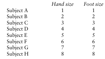
We can observe a perfect correlation between the size of the hands and the size of feet, from the person who has a size 1 hand and a size 1 foot to the person who has a size 8 hand and also a size 8 foot. There is a perfect positive correlation (as one variable increases, e.g. hand size, so the other variable—foot size—increases, and as one variable decreases so does the other).

Using a mathematical formula (a correlation statistic, available in most statistics books) we would calculate that this perfect correlation yields an index of association—a co-efficient of correlation—which is +1.00. Suppose that this time we carried out the investigation on a second group of eight people and reported the following results:

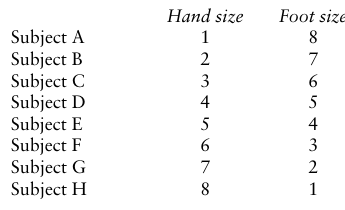
This time the person with a size 1 hand has a size 8 foot and the person with the size 8 hand has a size 1 foot. There is a perfect negative correlation (as one variable increases, e.g. hand size, the other variable—foot size—decreases, and as one variable decreases, the other increases). Using the same mathematical formula we would calculate that this perfect negative correlation yielded an index of association—a co-efficient of correlation—which is -1.00. Now, clearly it is very rare to find a perfect positive or a perfect negative correlation; the truth of the matter is that looking for correlations will yield co-efficient of correlation which lie somewhere between -1.00 and +1.00.

How do we know whether the co-efficient of correlation are significant or not? Let us say that we take a third sample of eight people and undertake an investigation into their hand and foot size. We enter the data case by case (Subject A to Subject H), indicating their rank order for hand size and then for foot size. This time the relationship is less clear because the rank ordering is more mixed, for example, Subject A has a hand size of 2 and 1 for foot size, Subject B has a hand size of 1 and a foot size of 2 etc.:

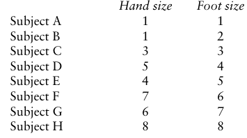
Using the mathematical formula for calculating the correlation statistic, we find that the coefficient of correlation for the eight people is 0.7857. Is it statistically significant? From a table of significance (commonly printed in appendices to books on statistics or research methods), we read off whether the co-efficient is statistically significant or not for a specific number of cases, for example:

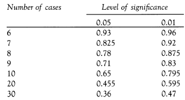
We see that for eight cases in an investigation the correlation co-efficient has to be 0.78 or higher, if it is to be significant at the 0.05 level, and 0.875 or higher, if it is to be significant at the 0.01 level of significance. As the correlation coefficient in the example of the third experiment with eight subjects is 0.7857 we can see that it is higher than that required for significance at the 0.05 level (0.78) but not as high as that required for significance at the 0.01 level (0.875).

We are safe, then, in stating that the degree of association between the hand and foot sizes rejects the null hypothesis and demonstrates statistical significance at the 0.05 level.

How Sample Size Affects Statistical Significance

The first example above of hands and feet (see p. 193) is very neat because it has 100 people in the sample. If we have more or less than 100 people how do we know if a relationship between two factors is significant? Let us say that we have data on 30 people; in this case, because our sample size is so small, we might hesitate to say that there is a strong association between the size of hands and size of feet if we observe that in 27 people (i.e. 90 per cent of the population).

On the other hand, let us say that we have a sample of 1,000 people and we observe the association in 700 of them. In this case, even though only 70 per cent of the sample demonstrates the association of hand and foot size, we might say that because the sample size is so large we can have greater confidence in the data than on the small sample. Statistical significance varies according to the size of the population in the sample (as can be seen also in the section of the table of significance reproduced above).

In order to be able to determine significance we need to have two facts in our possession: the size of the sample and the co-efficient of correlation. As the selection from the table of significance reproduced above shows, the co-efficient of correlation can de crease and still be statistically significant as long as the sample size increases. (This resonates with Krejcie and Morgan’s (1970) principles for sampling, observed, viz. as the population increases the sample size increases at a diminishing rate in addressing randomness.)

To ascertain significance from a table, then, it is simply a matter of reading off the significance level from a table of significance according to the sample size, or processing data on a computer programme to yield the appropriate statistic. In the selection from the table of significance for the third example above concerning hand and foot size, the first column indicates the number of people in the sample and the other two columns indicate significance at the two levels.

Hence, if we have 30 people in the sample then, for the correlation to be significant at the 0.05 level, we would need a correlation co-efficient of 0.36, whereas, if there were only 10 people in the sample, we would need a correlation co-efficient of 0.65 for the correlation to be significant at the same 0.05 level. In addition to the types of purpose set out above, the calculation of a correlation coefficient is also used in determining the item discriminability of a test, e.g. using a point bi-serial calculation, and in deter mining split-half reliability in test items using the Spearman rank order correlation statistic.

More recently statistical significance on its own has been seen as an unacceptable index of effect (Thompson, 1994, 1996, 1998; Thompson and Snyder, 1997; Rozeboom, 1997:335; Fitz Gibbon, 1997:43) because it depends on sample size. What is also required to accompany significance is information about effect size (American Psychological Association, 1994:18). Indeed effect size is seen as much more important than significance .

Statistical significance is seen as arbitrary and un helpful—a ‘corrupt form of the scientific method’ (Carver, 1978), being an obstacle rather than a facilitator in educational research. It commands slavish adherence rather than address ing the subtle, sensitive and helpful notion of effect size (see Fitz-Gibbon, 1997:118). Indeed commonsense should tell the researcher that a differential measure of effect size is more useful than the blunt edge of statistical significance.

Four Critical Caveats When Using Correlational Analysis

Whilst correlations are widely used in research, and they are straightforward to calculate and to interpret, the researcher must be aware of four caveats in undertaking correlational analysis:

1 Do not assume that correlations imply causal relationships (Mouly, 1978) (i.e. simply because having large hands appears to correlate with having large feet does not imply that having large hands causes one to have large feet).

2 There is a need to be alert to a Type I error— rejecting the null hypothesis when it is in fact true (a particular problem as the sample increases, as the chances of finding a significant association increase, irrespective of whether a true association exists (Rose and Sullivan, 1993:168), requiring the researcher, therefore to set a higher limit (e.g. 0.01 or 0.001) for statistical significance to be achieved).

3 There is a need to be alert to a Type II error—accepting the null hypothesis when it is in fact not true (often the case if the levels of significance are set too stringently, i.e. requiring the researcher to lower the level of significance (e.g. 0.1 or 0.2) required).

4 Statistical significance must be accompanied by an indication of effect size.

Identifying and resolving issues (2) and (3) are addressed earlier.

Linear vs. Curvilinear Correlations

What is Curvilinearity in Research?

The correlations discussed so far have assumed linearity, that is, the more we have of one property, the more (or less) we have of another property, in a direct positive or negative relationship. A straight line can be drawn through the points on the scatter diagrams (scatterplots). However, linearity cannot always be assumed. Consider the case, for example, of stress: a little stress might enhance performance (‘setting the adrenalin running’) positively, whereas too much stress might lead to a downturn in performance.

Where stress enhances performance there is a positive correlation, but when stress debilitates performance there is a negative correlation. The result is not a straight line of correlation (indicating linearity) but a curved line (indicating curvilinearity). This can be shown graphically (Box ). It is assumed here, for the purposes of the example, that muscular strength can be measured on a single scale. It is clear from the graph that muscular strength increases from birth until 50 years, and thereafter it declines as muscles degenerate.

There is a positive correlation between age and muscular strength on the left hand side of the graph and a negative correlation on the right hand side of the graph, i.e. a curvilinear correlation can be observed. Hopkins, Hopkins and Glass (1996:92) provide another example of curvilinearity: room temperature and comfort. Raising the temperature a little can make for greater comfort—a positive correlation—whilst raising it too greatly can make for discomfort—a negative correlation.

Many correlational statistics assume linearity (e.g. the Pearson product-moment correlation). However, rather than using correlational statistics arbitrarily or blindly, the researcher will need to consider whether, in fact, linearity is a reasonable assumption to make, or whether a curvilinear relationship is more appropriate (in which case more sophisticated statistics will be needed, e.g. η (‘eta’) (Glass and Hopkins, 1996, section 8.7; Cohen and Holliday, 1996:84) or mathematical procedures will need to be applied to transform non-linear relations into linear relations).

Common Examples of Curvilinear Relationships

Examples of curvilinear relationships might include:

Pressure from the principal and teacher performance;
Pressure from the teacher and student achievement;
Degree of challenge and student achievement;
Assertiveness and success;
Age and muscular strength;
Age and physical control;
Age and concentration;
Age and sociability;
Age and cognitive abilities. Hopkins, Hopkins and Glass (ibid.) suggest that the variable ‘age’ frequently has a curvilinear relationship with other variables.

The authors also point out (p. 92) that poorly constructed tests can give the appearance of curvilinearity if the test is too easy (a ‘ceiling effect’ where most students score highly) or if it is too difficult, but that this curvilinearity is, in fact, spurious, as the test does not demonstrate sufficient item difficulty or discriminability. In planning correlational research, then, attention will need to be given to whether linearity or curvilinearity is to be assumed.

Advanced Correlation Techniques: Multiple and Partial Correlation

The co-efficient of correlation, then, tells us something about the relations between two variables. Other measures exist, however, which al low us to specify relationships when more than two variables are involved. These are known as measures of ‘multiple correlation’ and ‘partial correlation’. Multiple correlation measures indicate the degree of association between three or more variables simultaneously.

We may want to know, for example, the degree of association between delinquency, social class background and leisure facilities. Or we may be interested in finding out the relationship between academic achievement, intelligence and neuroticism.

What is Multiple Correlation?

Multiple correlation, or ‘regression’ as it is sometimes called, indicates the degree of association between n variables. It is related not only to the correlations of the independent variables with the dependent variables, but also to the intercorrelations between the de pendent variables.

Understanding Partial Correlation

Partial correlation aims at establishing the degree of association between two variables after the influence of a third has been controlled or partialled out. Studies involving complex relationships utilize multiple and partial correlations in order to provide a clearer picture of the relationships being investigated. Guilford and Fruchter (1973) define a partial correlation between two variables as: one that nullifies the effects of a third variable (or a number of variables) upon both the variables being correlated.

The correlation between height and weight of boys in a group where age is per mitted to vary would be higher than the correlation between height and weight in a group at constant age. The reason is obvious. Because certain boys are older, they are both heavier and taller. Age is a factor that enhances the strength of correspondence between height and weight. With age held constant, the correlation would still be positive and significant because at any age, taller boys tend to be heavier. (Guilford and Fruchter, 1973)

When to Use Correlational vs. Experimental Research

Correlational research is particularly useful in tackling problems in education and the social sciences because it allows for the measurement of a number of variables and their relationships simultaneously. The experimental approach, by contrast, is characterized by the manipulation of a single variable, and is thus appropriate for dealing with problems where simple causal relationships exist. In educational and behavioral research, it is invariably the case that a number of variables contribute to a particular outcome.

Experimental research thus introduces a note of unreality into research, whereas correlational approaches, while less rigorous, allow for the study of behaviour in more realistic settings. Where an element of control is required, however, partial correlation achieves this without changing the context in which the study takes place. However, correlational research is less rigorous than the experimental approach because it exercises less control over the independent variables; it is prone to identify spurious relation patterns; it adopts an atomistic approach; and the correlation index is relatively imprecise, being limited by the unreliability of the measurements of the variables.

Types of Correlational Studies

Correlational studies may be broadly classified as either ‘relational studies’ or as ‘prediction studies’. We now look at each a little more closely.

Relational Studies: Exploring Variable Relationships

In the case of the first of these two categories, correlational research is mainly concerned with achieving a fuller understanding of the complexity of phenomena or, in the matter of behavioral and educational research, behavioral patterns, by studying the relationships between the variables which the researcher hypothesizes as being related. As a method, it is particularly useful in exploratory studies into fields where little or no previous research has been under taken. It is often a shot in the dark aimed at verifying hunches a researcher has about a presumed relationship between characteristics or variables.

Take a complex notion like ‘teacher effectiveness’, for example. This is dependent upon a number of less complex factors operating singly or in combination. Factors such as intelligence, motivation, person perception, verbal skills and empathy come to mind as possibly having an effect on teaching outcomes. A review of the research literature will confirm or reject these possibilities. Once an appropriate number of factors have been identified in this way, suitable measures may then be chosen or developed to assess them.

They are then given to a representative sample and the scores obtained are correlated with a measure of the complex factor being investigated, namely, teacher effectiveness. As it is an exploratory undertaking, the analysis will consist of correlation coefficients only, though if it is designed carefully, we will begin to achieve some understanding of the particular behaviour being studied. The investigation and its outcomes may then be used as a basis for further research or as a source of additional hypotheses.

Exploratory relationship studies may also employ partial correlational techniques. Partial correlation is a particularly suitable approach when a researcher wishes to nullify the influence of one or more important factors upon behaviour in order to bring the effect of less important factors into greater prominence. If, for example, we wanted to understand more fully the determinants of academic achievement in a comprehensive school, we might begin by acknowledging the importance of the factor of intelligence and establishing a relationship between intelligence and academic achievement.

The intelligence factor could then be held constant by partial correlation, thus enabling the investigator to clarify other, lesser factors such as motivation, parental encouragement or vocational aspiration. Clearly, motivation is related to academic achievement but if a pupil’s motivation score is correlated with academic achievement without controlling the intelligence factor, it will be difficult to assess the true effect of motivation on achievement because the pupil with high intelligence but low motivation may possibly achieve more than pupils with lower intelligence but higher motivation.

Once intelligence has been nullified, it is possible to see more clearly the relationship between motivation and achievement. The next stage might be to control the effects of both intelligence and motivation and then to seek a clearer idea of the effects of other selected factors—parental encouragement or vocational aspiration, for instance. Finally, exploratory relationship studies may employ sophisticated, multivariate techniques in teasing out associations between dependent and independent variables.

Prediction Studies: Forecasting Future Behaviors

In contrast to exploratory relationship studies, prediction studies are usually undertaken in areas having a firmer and more secure knowledge base. Prediction through the use of correlational techniques is based on the assumption that at least some of the factors that will lead to the behaviour to be predicted are present and measurable at the time the prediction is made (see Borg, 1963). If, for example, we wanted to predict the probable success of a group of sales people on an intensive training course, we would start with variables that have been found in previous research to be related to later success in sales work.

These might include enterprise, verbal ability, achievement motivation, emotional maturity, sociability and so on. The extent to which these predictors correlate with the particular behaviour we wish to predict, namely, successful selling, will determine the accuracy of our prediction. Clearly, variables crucial to success cannot be predicted if they are not present at the time of making the prediction. A sales-person’s ability to fit in with a team of his or her fellows cannot be predicted where these future colleagues are unknown.

In order to be valuable in prediction, the magnitude of association between two variables must be substantial; and the greater the association, the more accurate the prediction it permits. In practice, this means that anything less than perfect correlation will permit errors in predicting one variable from knowledge of the other. Borg recalls that much prediction research in the United States has been carried out in the field of scholastic success.

Some studies in this connection have been aimed at short-term prediction of students’ performance in specific courses of study, while other studies have been directed at long-term prediction of general academic success. Sometimes, short-term academic prediction is based upon a single predictor variable. Most efforts to predict future behaviours, however, are based upon scores on a number of predictor variables, each of which is useful in predicting a specific aspect of future behaviour.

In the pre diction of college success, for example, a single variable such as academic achievement is less effective as a predictor than a combination of variables such as academic achievement together with, say, motivation, intelligence, study habits, etc. More complex studies of this kind, therefore, generally make use of multiple correlation and multiple regression equations. Predicting behaviours or events likely to occur in the near future is easier and less hazardous than predicting behaviours likely to occur in the more distant future.

The reason is that in short-term prediction, more of the factors leading to success in predicted behaviour are likely to be present. In addition, short-term prediction allows less time for important predictor variables to change or for individuals to gain experience that would tend to change their likelihood of success in the predicted behaviour.

One further point: correlation, as Mouly and Borg observe, is a group concept, a generalized measure that is useful basically in predicting group performance. Whereas, for instance, it can be predicted that gifted children as a group will succeed at school, it cannot be predicted with certainty that one particular gifted child will excel. Further, low co-efficient will have little predictive value, and only a high correlation can be regarded as valid for individual prediction.

How to Interpret Correlation Coefficients

Interpreting the correlation co-efficient Once a correlation co-efficient has been computed, there remains the problem of interpreting it.

Three Approaches to Interpreting Correlations

A question often asked in this connection is how large should the co-efficient be for it to be meaningful. The question may be approached in three ways: by examining the strength of the relationship; by examining the statistical significance of the relationship (discussed earlier); and by examining the square of the correlation co efficient. Inspection of the numerical value of a correlation co-efficient will yield clear indication of the strength of the relationship between the variables in question.

Low or near zero values indicate weak relationships, while those nearer to +1 or -1 suggest stronger relationships. Imagine, for instance, that a measure of a teacher’s success in the classroom after five years in the profession is correlated with her final school experience grade as a student and that it was found that r=+0.19. Suppose now that her score on classroom success is correlated with a measure of need for professional achievement and that this yielded a correlation of 0.65.

It could be concluded that there is a stronger relationship between success and professional achievement scores than between success and final student grade. Exploratory relationship studies are generally interpreted with reference to their statistical significance, whereas prediction studies depend for their efficacy on the strength of the correlation co-efficient. These need to be considerably higher than those found in exploratory relationship studies and for this reason rarely invoke the concept of significance. The third approach to interpreting a co-efficient is provided by examining the square of the co-efficient of correlation, r2. T

his shows the proportion of variance in one variable that can be attributed to its linear relationship with the second variable. In other words, it indicates the amount the two variables have in common. If, for example, two variables A and B have a correlation of 0.50, then (0.50)2 or 0.25 of the variation shown by the B scores can be attributed to the tendency of B to vary linearly with A. Box shows graphically the common variance between reading grade and arithmetic grade having a correlation of 0.65.

Common Mistakes When Interpreting Correlation Coefficients

There are three cautions to be borne in mind when one is interpreting a correlation co-efficient. First, a co-efficient is a simple number and must not be interpreted as a percentage. A correlation of 0.50, for instance, does not mean 50 per cent relationship between the variables. Further, a correlation of 0.50 does not indicate twice as much relationship as that shown by a correlation of 0.25. A correlation of 0.50 actually indicates more than twice the relationship shown by a correlation of 0.25.

In fact, as co-efficient approach +1 or -1, a difference in the absolute values of the co-efficient becomes more important than the same numerical difference between lower correlations would be. Second, a correlation does not necessarily imply a cause-and-effect relationship between two factors, as we have previously indicated. Third, a correlation co-efficient is not to be interpreted in any absolute sense. A correlational value for a given sample of a population may not necessarily be the same as that found in another sample from the same population.

Many factors influence the value of a given correlation coefficient and if researchers wish to extrapolate to the populations from which they drew their samples they will then have to test the significance of the correlation. We now offer some general guidelines for interpreting correlation co-efficient. They are based on Borg’s (1963) analysis and assume that the correlations relate to a hundred or more subjects.

Correlation Ranges: 0.20 to 0.35 (Slight Relationships)

Correlations within this range show only very slight relationship between variables although they may be statistically significant. A correlation of 0.20 shows that only 4 per cent of the variance is common to the two measures. Whereas correlations at this level may have limited meaning in exploratory relationship research, they are of no value in either individual or group prediction studies.

Correlation Ranges: 0.35 to 0.65 (Moderate Relationships)

Within this range, correlations are statistically significant beyond the 1 per cent level. When correlations are around 0.40, crude group pre diction may be possible. As Borg notes, correlations within this range are useful, however, when combined with other correlations in a multiple regression equation. Combining several correlations in this range can in some cases yield individual predictions that are correct within an acceptable margin of error. Correlations at this level used singly are of little use for individual prediction because they yield only a few more correct predictions than could be accomplished by guessing or by using some chance selection procedure.

Correlation Ranges: 0.65 to 0.85 (Strong Relationships)

Correlations within this range make possible group predictions that are accurate enough for most purposes. Nearer the top of the range, group predictions can be made very accurately, usually predicting the proportion of successful candidates in selection problems within a very small margin of error. Near the top of this correlation range individual predictions can be made that are considerably more accurate than would occur if no such selection procedures were used.

Correlation Ranges: Over 0.85 (Very Strong Relationships)

Correlations as high as this indicate a close relationship between the two variables correlated. A correlation of 0.85 indicates that the measure used for prediction has about 72 per cent variance in common with the performance being predicted. Prediction studies in education very rarely yield correlations this high. When correlations at this level are obtained, however, they are very useful for either individual or group prediction.

Real-World Examples of Correlational Research

To conclude this blog post, we illustrate the use of correlation co-efficient in a small-scale study of young children’s attainments and self-images, and, by contrast, we report some of the findings of a very large scale, longitudinal survey of the outcomes of truancy that uses special techniques for controlling intruding variables in looking at the association between truancy and occupational prospects. Finally, we show how partial correlational techniques can clarify the strength and direction of associations between variables Small-scale study of attainment and self-image.

Case Study 1: Children’s Self-Assessment and Academic Achievement

A study by Crocker and Cheeseman (1988) investigated young children’s ability to assess the academic worth of themselves and others. Specifically, the study posed the following three questions:

1 Can children in their first years at school assess their own academic rank relative to their peers?

2 What level of match exists between self-estimate, peer-estimate, teacher-estimate of academic rank?

3 What criteria do these children use when making these judgements?

Using three infant schools in the Midlands the age range of which was from 5 to 7 years, the researchers selected a sample of 141 children from 5 classes. Observations took place on 20 half-day visits to each class and the observer was able to interact with individual children.

Notes on interactions were taken. Subsequently, each child was given pieces of paper with the names of all his or her classmates on them and was then asked to arrange them in 2 piles—those the child thought were ‘better than me’ at school work and those the child thought were ‘not as good as me’. No child suggested that the task was one which he or she could not do.

The relative self-rankings were converted to a percentage of children seen to be ‘better than me’ in each class. Correspondingly, each teacher was asked to rank all the children in her class without using any standardized test. Spearman’s rank order correlations were calculated between self-teacher, self-peer, and peer-teacher rankings. The table below indicates there was a high degree of agreement between self-estimates of rank position, peer estimate and teacher estimate.

The correlations appeared to confirm earlier researches in which there was broad agreement between self, peer and teacher ratings. The researchers conclude that the youngest schoolchildren quickly acquire a knowledge of those academic criteria that teachers use to evaluate pupils. The study disclosed a high degree of agreement between self, peers and teacher as to the rank order of children in a particular classroom. It seemed that only the youngest used nonacademic measures to any great extent and that this had largely disappeared by the time the children were 6 years old.

Case Study 2: Truancy and Long-Term Employment Outcomes

Drawing on the huge database of the National Child Development Study (a longitudinal sur vey of all people in Great Britain born in the week 3–9 March, 1958), Hibbett and her associates (1990) were able to explore the association between reported truancy at school, based on information obtained during the school years, and occupational, financial and educational progress, family formation and health, based on interview at the age of 23 years. We report here on some occupational outcomes of truancy.

Whereas initial analyses demonstrated a consistent relationship between truancy and drop ping out of secondary education, less skilled employment, increased risk of unemployment and a reduced chance of being in a job involving further training, these associations were de rived from comparisons between truants and all other members of the 1958 cohort. In brief, they failed to take account of the fact that truants and no truants differed in respect of such vital factors as family size, father’s occupation, and poorer educational ability and attainment before truancy commenced.

Using sophisticated statistical techniques, the investigators went on to control for these initial differences, thus enabling them to test whether or not the outcomes for truants differed once they were being compared with people who were similar in these respects. The multivariate techniques used in the analyses need not concern us here. Suffice it to say that by and large, the differences that were noted before controlling for the intruding variables persisted even when those controls were introduced. That is to say, truancy was found to correlate with:

unstable job history;
a shorter mean length of jobs;
higher total number of jobs;
greater frequency of unemployment;
greater mean length of unemployment spells;
lower family income.

Thus, by sequentially controlling for such variables as family size, father’s occupation, measured ability and attainment at 11 years, etc., the researchers were able to ascertain how much each of these independent variables contributed to the relationship between truancy and the outcome variables that we identify above. The investigators report their findings in terms such as:

truants were 2.4 times more likely than non-truants to be unemployed rather than in work;
truants were 1.4 times more likely than non-truants to be out of the labor force;
truants experienced, on average, 4.2 months more unemployment than non-truants;
truants were considerably less well off than non-truants in net family income per week.

The researchers conclude that their study challenges a commonly held belief that truants simply outgrow school and are ready for the world of work. On the contrary, truancy is often a sign of more general and long-term difficulties and a predictor of unemployment problems of a more severe kind than will be the experience of others who share the disadvantaged backgrounds and the low attainments that typify truants.

Case Study 3: Teacher Training and Student Performance

The ability of partial correlational techniques to clarify the strength and direction of associations between variables is demonstrated in a study by Halpin, Croll and Redman (1990). In an exploration of teachers’ perceptions of the effects of in-service education, the authors report correlations between Teaching (T), Organization and Policy (OP), Attitudes and Knowledge (AK) and the dependent variable, Pupil Attainment (PA).

The strength of these associations suggests that there is a strong tendency (r=0.68) for teachers who claim a higher level of ‘INSET effect’ on the Teaching dimension to claim also a higher level of effect on Pupil Attainment and vice versa. The correlations between the Organization and Policy (OP) and Pupil Attainment (PA), and Attitudes and Knowledge (AK) and Pupil Attainment (PA), however, are much weaker (r=0.27 and r=0.23 respectively). When the researchers calculated the partial correlation between Teaching and Pupil Attainment, controlling for:

(a) Organization and Policy

(b) Attitudes and Knowledge, the results showed little difference in respect of Teaching and Pupil Attainment (r=0.66 as opposed to 0.68 above).

However there was a noticeably reduced association with regard to Pupil Attainment and Organization and Policy (0.14 as opposed to 0.27 above) and Attitudes and Knowledge (0.09 as opposed to 0.23 above) when the association between Teaching and Pupil Attainment is partialled out. The authors conclude that improved teaching is seen as improving Pupil Attainment, regardless of any positive effects on Organization and Policy and Attitudes and Knowledge.

FAQs

What is the difference between correlation and causation?

Answer: Correlation measures the relationship between two variables, but it does not prove that one causes the other. For example, large hands may correlate with large feet, but having large hands doesn’t cause large feet. Both are influenced by other factors like genetics and overall body size. Always remember: correlation does not imply causation.

What is a good correlation coefficient in research?

Answer: The interpretation depends on your research purpose. For exploratory studies, correlations between 0.35-0.65 can be meaningful. For prediction studies, you’ll need higher correlations (0.65-0.85 or above) for accurate forecasting. Generally, correlations below 0.35 show weak relationships, while those above 0.85 indicate very strong relationships between variables.

How does sample size affect correlation significance?

Answer: Larger sample sizes require smaller correlation coefficients to achieve statistical significance. For example, with 10 subjects, you need a correlation of 0.65 for 0.05 significance, but with 30 subjects, you only need 0.36. This is because larger samples provide more reliable data and reduce the impact of random chance.

When should I use partial correlation instead of simple correlation?

Answer: Use partial correlation when you want to examine the relationship between two variables while controlling for the effect of a third variable. For instance, if studying the relationship between motivation and academic achievement, you might want to control for intelligence to see motivation’s true effect independent of cognitive ability.

https://nurseseducator.com/high-fidelity-simulation-use-in-nursing-education/

First NCLEX Exam Center In Pakistan From Lahore (Mall of Lahore) to the Global Nursing

Categories of Journals: W, X, Y and Z Category Journal In Nursing Education

AI in Healthcare Content Creation: A Double-Edged Sword and Scary

Social Links:

https://www.facebook.com/nurseseducator/

https://www.instagram.com/nurseseducator/

https://www.pinterest.com/NursesEducator/

https://www.linkedin.com/company/nurseseducator/

https://www.linkedin.com/in/nurseseducator/

https://www.researchgate.net/profile/Afza-Lal-Din

https://scholar.google.com/citations?hl=en&user=F0XY9vQAAAAJ